Chapter 2: Implementation
In this section, we will discuss the gory details that make quantum computing difficult to implement physically. We will then examine some of the many different architectures that are being developed for future quantum computers and compare their relative strengths and weaknesses.
A warning: Moreso than the previous section, the information contained here may go out of date. It’s possible that some of these technical approaches will become dominant, and others will lead to intellectual dead-ends. Progress in these fields is actively occurring, and in some cases, moving rather fast. As such, while I will describe the current state of the field, I will focus on the basics – e.g. how does a superconducting transmon qubit work, rather than the details of Google’s Willow superconducting quantum processor.
Qubits in Practice, Not Theory
Recall our discussion from Chapter 1 regarding classical bits: We currently implement these bits as voltage levels, stored in memory and processed by logic gates implemented by transistors in silicon. This is a choice informed by decades of semiconductor engineering, but it is equally possible (however much less scalable) to implement classical bit-based computation using light switches, tanks of water, or cans of soup. Anything where we can encode two different levels (logical 1 and logical 0) can be used as a bit. The trouble of course, is interacting with those bits in a scalable way: we’ve settled on transistors because we can create billions of them and easily control them.
Qubits are a bit more… finicky. Our qubits need several unique properties: superposition & entanglement. Unfortunately for quantum computer engineers, most things around us don’t seem to obey quantum properties on the macro- scale. I can’t put my light switch in a superposition! So we have to look for specific qubit ‘platforms’ which have a quantum nature. This naturally leads us to several of the most promising qubit technologies: photons, atoms, & ions. The last of the big four implementations is superconducting qubits, which exist on a larger, non-atomic scale, but utilize the properties of supercooled semiconductors to access quantum effects.
In each of these cases, we have to encode the state of the qubit ($\ket{0}$ or $\ket{1}$) in some specific physical property of the qubit. This could be the spin of the photon, the frequency of some vibration, or the energy of the system. This varies in each of the platforms, as does the mechanism of interacting with the system (implementing gates and measurement).
Fragile Qubits
Real-world qubits are inherently fragile. While I can turn my laptop off for several months and expect to come back to the system in the same state with my data uncorrupted, it’s a tall order for a qubit to last seconds in the same state. We know definitionally that quantum states can be affected (collapsed) by outside measurement. It’s not a very far leap to say that those quantum states can be similarly affected by any interaction with the outside world.* We can spend a lot of time precisely engineering the qubit system and still have our qubits end up in different, unknown states. This is called ‘decoherence’, and a critical metric for any quantum computer is how long a qubit can last before decoherence occurs. You’ll often actually see two relevant metrics for decoherence times, known as $T_1$ and $T_2$. $T_1$ is the time a qubit can stay in the $\ket{1}$ state, before it drops back down into the lower-energy $\ket{0}$ state. $T_ 2$ relates to the phase coherence of a state – i.e. how long can it last in a specific phase before that information is lost. Clearly, engineers would like to maximize both values to create stable, long-lived qubits.
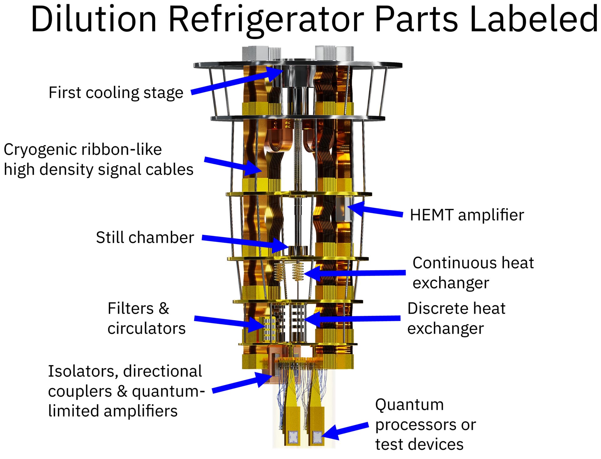
This also explains why lots of quantum computers need to be supercooled or placed into a vacuum: They want to avoid heat and interference from their environment! There’s a popular misconception that the massive, upside-down steel cylinders shown in press photographs and Fig. 1 are computers themselves, when they are just dilution refrigerators, specifically used for cooling superconducting quantum computers to tens of milli-Kelvin. These fridges have concentric inner partitions that progressively cool the system down to the working temperature. In other qubit hardware implementations, that temperature varies, but it is typical for the system to require some level of cooling, vacuum, or isolation from the environment.

But even with careful engineering, noise will occur. Our wonderful little qubits will begin to decohere, and the state that they we think they are in may not be the state they are actually in. And here, we get to potentially the most vexing, complicated, and misunderstood topic in all of quantum computation: error correction.
Qudits
We’re about to start talking about real world systems that we use to implement the theoretical concepts we call qubits. In each case, there is some property of the system that exhibits quantum behavior as it transitions between some set of states. In some cases, it may be that the quantum system can exist in more than two states. In those cases, one state will be assigned to $\ket{0}$, and another to $\ket{1}$. Those other states are typically considered undesirable leakage states. However, there is some interest in actually using those other states for computation.
The other states are labeled in bra-ket notation, and increment up from $\ket{1}$: $\ket{2}$, $\ket{3}$, etc. These systems are called ‘qudits’ (notice the D), after systems with ‘D’ levels. For this work, we won’t consider any qudit-based computation schemes, and all states greater than $\ket{1}$ are unwanted errors!
Error Correction Cliff Notes
I apologize. I’ve billed this section as being about the practical concerns of quantum computer implementation, and you’ve probably thought we would be talking about engineering problems. Real fun hardware implementation questions, with cool photos of semiconductors and atoms and lasers and the like. We will get to that, but first we need to do some more theory and math. You’re welcome to skip this section, but just know that error correction knowledge is what gives you real credibility on the mean streets out there. All the kids will laugh at you when you admit you don’t know what a qLDPC code is.
To save you embarrassment, I’m going to summarize all the important takeaways of error correction up front. In the next sub-section, we’ll do some math and familiarize ourselves with a surface code, but these are the practical concepts you should have in your mental model of error correction.
- To stop errors from occurring and propagating, we need to implement error correction. Error correction exists at the intersection of physical engineering and software protocol. It consists of rapidly repeating gates then measurement operations. Cumulatively they both detect and suppress errors.
- Errors may be introduced from the decoherence of individual qubits, noise from the environment, or from gate operations. As we’ll see, superconducting qubits are very sensitive, and require very aggressive error correction. Other qubit modalities, for example some implementations of trapped ions, have long coherence times and are more resistant to noise. Error correction is still necessary for those systems, because it’s very difficult to guarantee the accuracy of any particular gate operation. Certain companies are betting they can get away with doing less error correction than others, by virtue of their hardware platform's characteristics..
- Error correction is really tricky. In classical computing, we can just duplicate data. We can’t do that in a quantum computer, because of the ‘no-cloning’ rule (see Chapter 1). So instead, we encode a single qubit’s information across many qubits. This is why you’ll sometimes hear people talk about ‘physical qubits’ versus ‘logical qubits’. A logical qubit is comprised of many physical qubits, and we fundamentally care about logical qubits, because that’s what we do operations on. The physical/logical ratio varies based on the technological regime we are working in, but use something like 1000:1 as a rough guideline. Considering that current physical qubit counts are in the low hundreds, we have a long way to go.
- There are lots of different implementations of error correction. You’ll commonly see ‘surface codes’ and ‘color codes’. These are advantageous because they can be natively implemented on a grid of qubits, which is what superconducting and neutral atom systems naturally look like. However, there’s a lot of interest in ‘low density parity check’ (LDPC) codes. These codes can improve the physical/logical ratio, but can’t be implemented directly on a grid. Rather, they require being able to make qubits that aren’t immediately adjacent interact with each other. That’s easier for certain implementations, like ions & neutral atoms, where qubits can be physically moved around.
- Remember that a logical qubit doesn’t just look like X copies of the same physical qubit (because we literally could not do that with our current laws of physics). Instead, the data is sort of ‘broken apart’ across the physical qubits. That means that interacting with that data is not necessarily trivial. Ideally, to apply a gate to a logical qubit, we would just apply that gate to all of its constituent physical qubits – this is called a ‘transversal’ gate. Unfortunately, for any error correcting code, there will always be some gate that the system needs to be able to perform (i.e. part of the universal gate set) that cannot be done transversally. So no matter what, some gates will always be hard to implement on a logical qubit.
- For surface codes in particular, it’s easy to perform Clifford gates ({CNOT, H, S}) on logical qubits, but full computation requires more than just Clifford gates. As a result, there’s a lot of concern and literature on how to generate ‘magic states’, which implement T gates (which let you do non-Clifford gates, enabling universal quantum computation). Thus you’ll see papers discussing how to do magic state ‘distillation’ and ‘cultivation’. This is one of the big rate limiting steps for practically implementing lots of algorithms. Different code implementations have different strengths: For example, color codes may be denser and faster to perform computations on, and LDPC codes may require fewer physical qubits.
- Error correction leans on some very important theoretical results that say that if physical qubit error rates can be kept low enough, then continuous error correction should be able to guarantee successful computation. Perhaps the most important experimental result of the last decade is Google’s paper that showed they were able to successfully decrease the logical qubit error rate below the physical qubit error rate, and that increasing code distance (essentially the physical/logical ratio) further decreased that rate. That single result alone validated an enormous amount of research on quantum error correction.
- Those theoretical results about error correction rely on some important assumptions that may not be practically true. It assumes:
- That errors are limited to phase and bit flip errors. Think of these as essentially just errors that move the state of the qubits around on the Bloch sphere – just like single qubit gates. Unfortunately, many physical qubits struggle with something called ‘leakage’. We discussed the principle of `qudits' briefly above: in real-world qubit implementations, a system may have more than two states (e.g. it may have $\ket{2}$, $\ket{3}$, and so on). Leakage occurs when one of our qubits accidentally slips out of the bottom two energy levels into some higher state. Error correction can’t handle these kinds of faults, so systems must be carefully engineered to prevent leakage.
- Errors are independent and uncorrelated. This is troublesome. Lots of plausible error-causing mechanisms, like radiation coming in from the outside world , might create correlated errors in many qubits at a time. For quantum computation to last hours to days, these issues will have to be mitigated.
- When running these error correcting codes, there are data qubits (which store the actual data) and ancilla qubits (which give us information about the state of the data qubits). The code requires lots of repeated measurements of the ancilla qubits, which we then need to translate into a guess about the occurrence of errors in the system. There is not an obvious and easy way to ‘decode’ the measured information into error information. Even in the best case, there is uncertainty about what kind of error has (or hasn’t occurred), and implementing this process at high speed may require heuristic or machine learning inspired methods. NVIDIA has just thrown their hat into this ring with their announcement of their `Ising models' for decoding. This is a huge problem and an active field of research.
- You may have noticed that most of my citations and examples here come from Google’s quantum program. This is because they seem to be furthest along when it comes to practical implementation of error correction (and are certainly one of the teams most open about their results here). This isn’t to say that superconducting qubits (Google’s primary chosen modality) are the definitive best choice for future development, but rather that they are one of the farthest along in current development.
Phew. That was a lot of information! Let’s take a breather and learn some error correction theory.
Error Correction 101
Practically speaking, in classical computation, bits don’t fail that often. The most common rationale for a bit being corrupted (a 0 turning into a 1, or vice versa) is due to radiation. This is generally not a concern for most applications but it is an issue for electronics that operate in the upper atmosphere or space. Thus, we often see error correction & mitigation used in aerospace applications.
The simplest way of doing this is redundancy. If we want to store a value, we will instead store three copies of the same value. This is the simplest possible error correcting ‘code’. A ‘1’ becomes mapped to ‘111’, and ‘0’ becomes mapped to ‘000’. Note that in typical binary notation, 111 would mean 7, but we’ve changed its meaning here, because we’re representing our data in a different way. It’s very easy to see the original data we mean to store in this encoding, but that won’t always be the case.
If an error occurs, what happens? Let’s say we have a logical 1, which is encoded via the actual bit values ‘111’. A beam of radiation comes in and flips the middle bit. Now our bits look like ‘101’, which doesn’t have a clear logical value in our encoding. We use something called a ‘syndrome’ to figure out what logical value our computer should use. In this case, the syndrome essentially performs a majority vote – two of our bits say 1, and one says 0, so we should use 1. This was correct in this instance, but let’s say a beam of radiation hits ‘111’ and flips two bits, and we are left with ‘100’. Now our syndrome would report logical 0, the incorrect value. Any error correcting code is only resilient to a certain amount of error. The strength of a code is expressed via its ‘code distance’. A repetition code like this has distance 3, and can correct 1 error. If we encoded each logical bit using 5 normal bits (0 $\rightarrow$ 00000; 1 $\rightarrow$ 11111), the code could correct two errors at a time.
Note that I’ve described this process as a ‘majority vote’ but this would actually be implemented with what’s called a ‘parity check’. A parity check simply checks if two adjacent bits are the same value. For our three bit code, we’d do two parity checks, between the first and second bit and between the second and third bit. If both parity checks are clean, there is no error detected. If either or both parity checks reports a difference, we can flip a bit to make them all the same parity. Something important to see is that in this scheme, the checks don’t care about the actual value of the bits, just about their relative parity. This is important because in quantum-land, if we measure a qubit directly, we collapse its state. However, if we can implement our syndrome using a parity check function that indirectly compares the relative states of two qubits, we may be able to avoid direct measurement of those qubits.
Unfortunately, the errors that qubits experience are significantly harder to deal with than those of classical bits. A classical bit can flip from 0 to 1, or vice versa. A qubit can flip from $\ket{0}$ to $\ket{1}$, or to some intermediate value – we call these bit flip errors. Qubits can also have errors in their phase: $\ket{+}$ could flip to $\ket{-}$, or again to some intermediate degree. That would be a phase flip error. Thankfully, we can treat potentially intermediate analog errors (i.e. partial rotations on the Bloch sphere) as linear combinations of full phase or bit flip errors. As a result, we really can think just in terms of preventing discrete errors.
How might we begin to do this? Well, we could attempt to implement a repetition code for qubits. But there’s a problem. Remember the no-cloning theorem? We can’t just duplicate an arbitrary qubit state, i.e. turn $\ket{\psi}$ into $\ket{\psi}\ket{\psi}$. What we can do, is entangle a qubit with an ancilla qubit, and create some combined quantum state.
$$CNOT(\ket{\psi} \ket{0}) = CNOT((\alpha \ket{0} + \beta \ket{1}) \ket{0}) = \alpha\ket{00} + \beta\ket{11} = \ket{\psi_L}$$Note that this is not just $\ket{\psi}\ket{\psi}$! This is an entangled state, not two independent qubits. This new system is our logical qubit, which we will denote with subscript L. We say this is the ‘encoded’ state.
Now let’s say the qubits are at risk of a bit flip error (we can call this an X error, since it looks like applying an X gate). How do we figure out (and try to correct) that error? Well, we need to measure the qubits. But remember, measuring either of the constituent physical qubits directly would collapse the system’s state, losing information. So what we do is akin to the parity check described above in the context of classical error correction. We take another qubit (an ancilla) and perform two conditional Z measurements on it, one for each of the two physical qubits in our logical qubit. These measurements are called the stabilizer. Why? Well, as we’ll see, performing the stabilizer measurements actually reduces the probability of an error propagating through the system.
We then measure the ancilla, and the system (which consists of three entangled qubits) collapses to one of two states. That measured value is our syndrome, which we use to decode the error. If the error has a $p_x = a_x^2$ chance of occurring per qubit (and a $(1-p_x) = k_1^2$ chance of not occurring, we can express the state of the system as:
$$(k_1^2 + k_x^2 X_1 X_2) \ket{\psi_L}\ket{0} + k_1 k_x (X_1 + X_2) \ket{\psi_L}\ket{1} $$If the ancilla ends up in $\ket{1}$, that indicates that the qubits are not the same parity, and a bit flip error has occurred. If the ancilla is measured to be $\ket{0}$, then the two data qubits will collapse to being the same parity – this either means no error has occurred, or both qubits have experienced a bit flip (2 errors!). Notice that even in this very simple example, we still have uncertainty about the state of the system, and cannot cleanly map our syndrome to an error (or lack thereof). We can do the math to figure out the probability of the system being in that double bit flipped state. It turns out that conditional on measuring $\ket{0}$, there’s only a $p_x^2$ chance of error remaining in the system. That means that this code, specifically the application of the stabilizer, does suppress errors in the system.
Let’s identify two other practical issues with using this code: First, if we do detect an error, we can’t really correct it! We don’t know which of the two qubits was the one that experienced the bit flip error. This makes this more of an error detecting code than an error correcting code. Second, we can only check for bit flip errors, not phase flip errors. We can rectify both these issues by, you guessed it, adding more qubits.
There are many families of error correcting codes (we discussed color codes and LDPC codes in our quick highlights above), but the most mature are the surface codes. Surface codes have natural advantages in that they naturally can be implemented on a grid of qubits, requiring only nearest-neighbor interactions on a square grid. I’m not going to cover surface codes in depth, but we can look at a very high level example of how they are implemented.
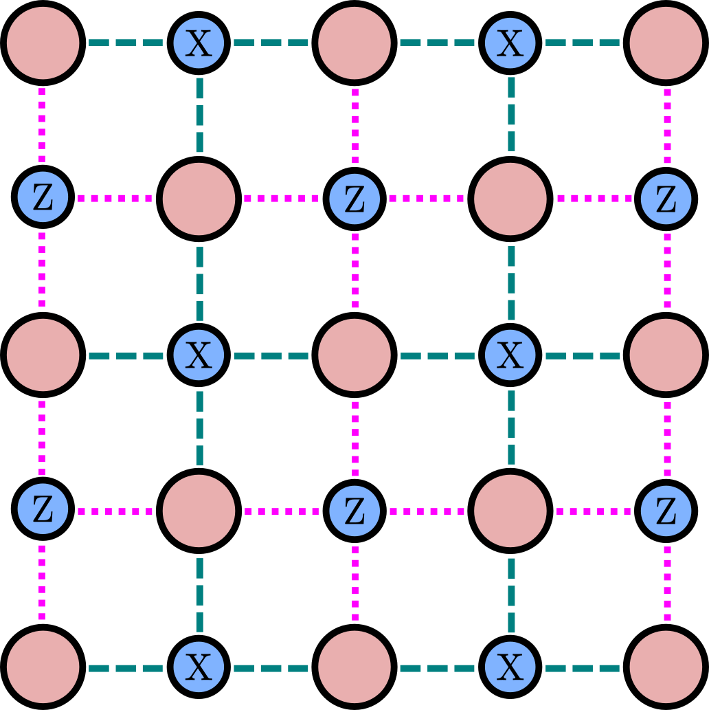
Figure 2 shows a grid of qubits, alternating between data and ancilla in a checkerboard pattern. The logical qubit’s data is broken apart across the states of all the data qubits, and the error code is implemented via stabilizer measurements (conditional Z and X’s) on the ancilla qubits. Each ancilla checks against either bit or phase flip errors, and only gets one kind of measurement projected on it. The surface code is implemented in cycles, where each ancilla gets a conditional gate from each of its neighboring nodes, then a measurement occurs. There are a lot of funky implementation details (such as, what order to do these gates in), but this is the general schema. Once again, note that the measurements of the ancilla do not generally translate directly into concrete information about what errors have occurred, and there is computational effort that must be expended trying to ‘decode’ the errors.
We’ve now understood a few fundamental principles about quantum error correction. I’ve done a big summary above, but I want to emphasize a few points as we begin to discuss physical qubit implementations. Error is an inherent part of quantum computation, and successful quantum computers will design qubits to incur as few errors as possible in the first place, while implementing active error correction schemes which are continuously fixing the errors that do occur. This is a tremendously difficult problem, and informs nearly every aspect of qubit engineering and system design.
Quantum Skepticism
This feels like an appropriate time to acknowledge that some people simply don’t think building a fault tolerant quantum computer is possible. I think there is a spectrum to the validity of these doubts, so I’d like to present a few different common critiques and explain their perspectives.
The most common and perhaps least sound skepticism is the common refrain ‘Why haven’t quantum computers factored 35 yet?’, often dropped below any quantum computing-related internet post. The idea being, if quantum computers are so powerful, why haven’t we seen evidence of their ability to do tasks that would be trivial for typical computers? We’ve already discussed the difficulty of implementing Shor’s algorithm above; so it’s no surprise that today’s small scale and limited quantum computers are unable to factor large numbers. I find this argument incredibly unpersuasive: Everyone in the field knows that today’s devices are simply not performant enough! If we had thousands of qubits and working error correction and still couldn’t factor 35, that would be a different story. Craig Gidney argues that we might expect error correction performance to follow an exponential trendline - this would similarly imply nonlinear growth in actual computational capabilities. So I think this is a lousy and intellectually lazy tack!
An alternative critique says: “These quantum computers are simply too hard/impossible to build!” This paper is a very representative example. On some level, it’s difficult to engage with this line of argument, since there are any number of characteristics of a quantum computer which are incredibly difficult to implement (qubit count, control, gate fidelity, interconnections, error correction schemes, syndrome decoding, etc. etc.). Certainly there are those who thought the systems of today (100+ qubits implemented across several different kinds of physical platforms) would have been impossible. At the same time, the remaining challenges in scaling up to thousands and eventually millions of qubits seem daunting and perhaps insurmountable. There is no guarantee that these problems can be solved, but nor is there a guarantee that they cannot. So, I think this critique is potentially, but not necessarily, true. It most definitely is not a reason to abandon development!
Lastly, I want to highlight the perspective of Israeli mathematician Gil Kalai, who’s often cited as one of the most prominent and vocal quantum computing skeptics. Gil’s point of view is essentially that there will be some level of correlated noise in quantum systems that error correction schemes will not be able to mitigate. Once again, this is difficult to prove or disprove. Existing error correction experiments have not yet hit this limit, but it is entirely possible, but perhaps not plausible, that they may one day, neutering efforts to reach full fault tolerant operation.
Personally, I find elements of these arguments compelling, and as a natural skeptic I am sympathetic to their claims. In particular, I think scaleup is an extremely difficult problem for just about every hardware platform being produced, one that may cull a great number of quantum hardware companies in the near future. I can’t quite sit in the quantum computing isn’t possible camp, though. As we are about to see, the field has come a long way in physically implementing qubits, and the influx of interest and funding could lead to even more rapid progress.
Physical Qubit Implementations
And now we arrive at my favorite section: Understanding how qubits actually get built. In the following sections, we will look at several leading architectures for qubit implementations. In each, we will attempt to answer a few important questions:
- How is a qubit encoded in this physical system?
- How is the state of a qubit (or qubits) changed – i.e. how do we perform 1 and 2 qubit gate operations?
- How do we measure our qubits?
- What does the full system look like?
- What are the relative strengths or weaknesses of this approach relative to the others?
Superconducting
We begin with superconducting qubits. This approach is probably the most mature, with a relatively long lineage of academic work bolstered by significant investment from tech giants like Google and IBM. As previously mentioned, Google’s Quantum AI team has some of the most impressive announced results in both hardware (qubit counts & fidelity) and software (algorithms with realized quantum advantage, implemented on their hardware).
Unfortunately, in many regards, superconducting qubits are also the modality that is most difficult to understand. Of my listed ‘Big 4’ (superconducting, atoms, ions, photons), superconducting qubits are the only one not using a basic physical particle – something you might learn about in high school chemistry class. The layman knows what an atom is, but not what a ‘transmon’ is. Thankfully, we can build up a physical intuition for the superconducting qubit without too much trouble. Even better, we can re-use much of this intuition when we examine the other types of qubit implementations.
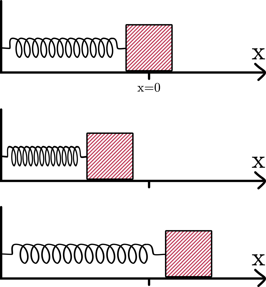
Before we talk about superconductors, silicon, quantum states, or anything else, we’re going to go back to high school physics. Consider, as in Fig. 3, a mass mounted to a spring, in turn mounted to a fixed point. The mass is frictionless and does not lose energy as it slides across the ground – it’s ideal! If we put energy into this system, it will oscillate forever. This is usually a bad assumption for the real world, but in fact is a great assumption for the world of superconductors: These conductors are so ‘super’ because they don’t dissipate energy. A copper wire at room temperature is a pretty good conductor (certainly better than air, or wood, or rubber), but has finite resistance. If I induce some current in a loop of copper, it will generate heat and die out. Not so in a superconductor! Superconducting qubits utilize metals which exhibit superconductivity at very low temperatures (single digit Kelvin, just above absolute zero). That’s an important reason why these qubits are kept in dilution fridges.
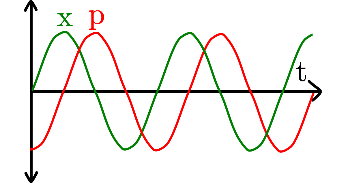
I digress! We are just talking about springs and masses. We’re going to care about a few properties of the system: its energy, position, and momentum (which is equivalent to its velocity). If the system is sitting still: there’s zero energy and zero momentum, and we will call this position zero. If we perturb the system, it will oscillate! The energy in the system will slosh back and forth between the mass's position and its momentum. When the position reaches an extreme, the instantaneous velocity & momentum will be zero. Conversely, when the position is zero, the instantaneous momentum will be at its highest. We can graph position versus time and momentum versus time, and get two out of phase sine waves. We can also graph position versus momentum, and get a circle, as in Fig. 4.
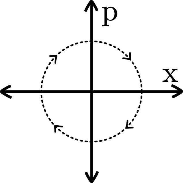
In each of these cases, if we perturb the system more and put additional energy into it, the amplitudes of the sines get bigger – i.e. higher energy means larger peak momentum and position. We can add energy to that position vs. momentum graph and get a conical shape in 3D. We can then take a cross section of that cone to see position versus energy, getting a parabolic shape, shown in Fig. 5.
OK! That was a lot of preamble to say something very simple: If a mass on a spring has a position far away from its equilibrium point, it has more energy! Now… let’s make the system scarier… instead of a mass on a spring… let's imagine a quantum mass on a quantum spring. Everything is very very tiny, and obeys the laws of quantum physics. What changes? First and foremost, our energy levels are quantized. Depending on your level of familiarity with quantum physics, this may be a given or incredibly confusing. The following explanation is a gross oversimplification (sorry real physicists), but it is helpful: As we get to very small particles and systems, nature becomes discrete, not continuous. Our system can have 1 unit of energy, or 2 units of energy, but not 1.5 units of energy. It can only sit in certain discrete states. We can show this by drawing lines on our parabola, each representing a valid quantum state. We will also label each state with our special bra-ket notation.
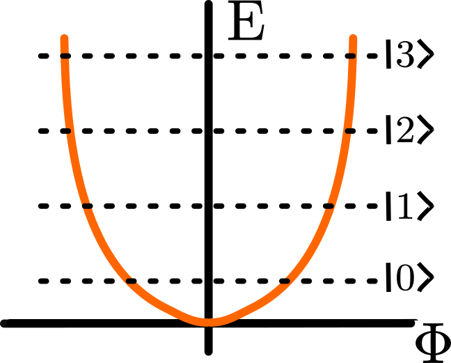
I mentioned this before, but it bears repeating. This system has more than 2 states! So while we pick the bottom two states to be $\ket{0}$ and $\ket{1}$, we also have $\ket{2}$ through $\ket{N}$ other states. Almost always, we don’t actually want our computer to be in those states, as that can cause uncorrectable errors. It’s very important for our system to be limited to states $\ket{0}$ and $\ket{1}$.
One more quantum property we care about: the system is now probabilistic. We cannot directly measure its velocity and its position at the same time, due to Heisenberg’s famous uncertainty principle. As such, we can’t have total certainty about the state that it’s in. To make an analogy to a truly classical system: If we could only measure the position of the mass on a spring, observing it as position zero means it’s likely in a lower energy state, but it could be the mass briefly and rapidly moving through center position as it oscillates while in a higher energy state. We simply can’t be sure!
This is confusing, but should be a bit more intuitive given that you’ve just read quite a bit about probabilistic models of computation. Just keep in mind that just like our theoretical qubits from section 1, we can put the system into superpositions of states and that, upon measurement, the system will collapse to a singular valid quantized state.
Let’s now put our microscopic mass and spring into a dilution fridge, and cool it down to 40 millikelvin. Brrr! It ends up being in its ground state - $\ket{0}$. There’s virtually no motion. How do we excite the system – i.e., move it from $\ket{0}$ to $\ket{1}$? We have to inject some energy. In the mass and spring example, we’d have to give it a very careful, precisely calibrated microscopic tap. After all, we want to be in $\ket{1}$, not $\ket{2}$ or $\ket{3}$. Keep this in mind as we move forward.
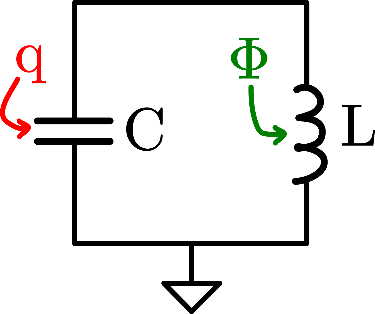
Unfortunately, we are running into the useful limits of our mass and spring resonator example. We can keep most of our mental model the same, but we need to introduce how these systems are actually built – with electronic circuit elements. We are going to substitute our mass and spring for an inductor and a capacitor in parallel. These are two circuit elements that store energy. The capacitor is represented by two parallel lines, and the inductor by a coiled line. A capacitor stores energy in an electric field (often between two parallel plates of conductive material) and an inductor stores energy in a magnetic field generated by current running through loops of conductors. While we are drawing them as symbols in our little circuit model, these are in fact physical objects that we can design and manufacture by depositing or etching metal in certain shapes on a silicon wafer.
The inductor and capacitor form what is known as an LC oscillator. At a certain frequency (called the resonant frequency, determined by the value of each of the components), energy perfectly sloshes back and forth between the inductor and the capacitor. It is directly analogous to the mass on a spring, where energy moves back and forth between the momentum of the mass and the potential energy in the compressed or stretched spring. We can reuse the diagrams from before and just change the variables from position (x) and momentum (p) to flux in the inductor ($\Phi$) and charge on the capacitor ($q$). We’ve changed our physical example, but ended up in the same place.
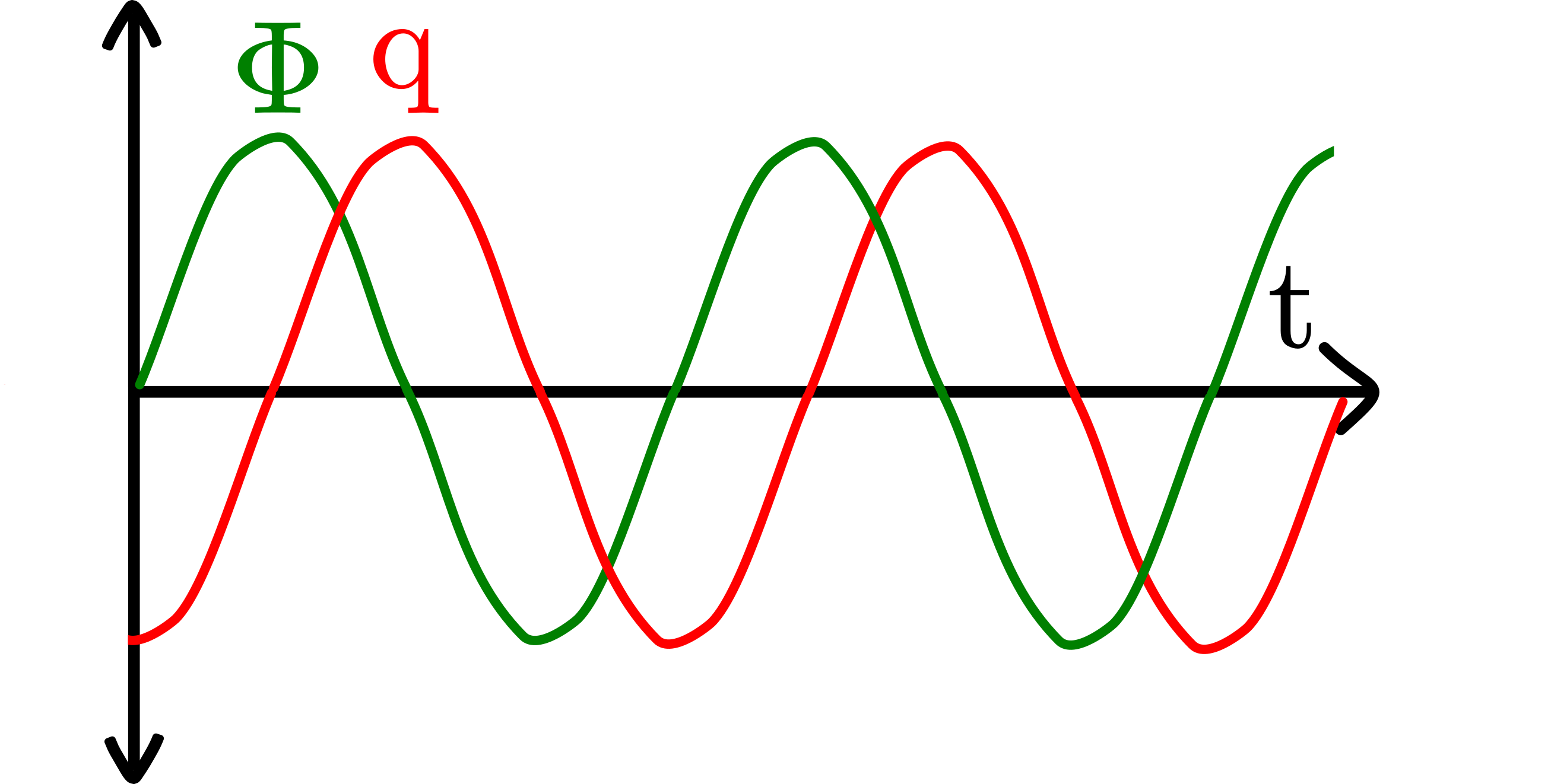
Now, if we want to excite the system, we need to add some energy into it. We do this by blasting the oscillator with some high frequency microwave radiation. This is roughly the same as putting leftovers into your microwave and having the water inside be excited at its resonant frequency, heating the meal up. Importantly, the system only wants to resonate at a certain frequency (its resonance), so we have to tune the waves to excite the system at that frequency. Again, based on certain properties of the oscillator, we can figure out what that frequency needs to be. So we are almost at the qubit!
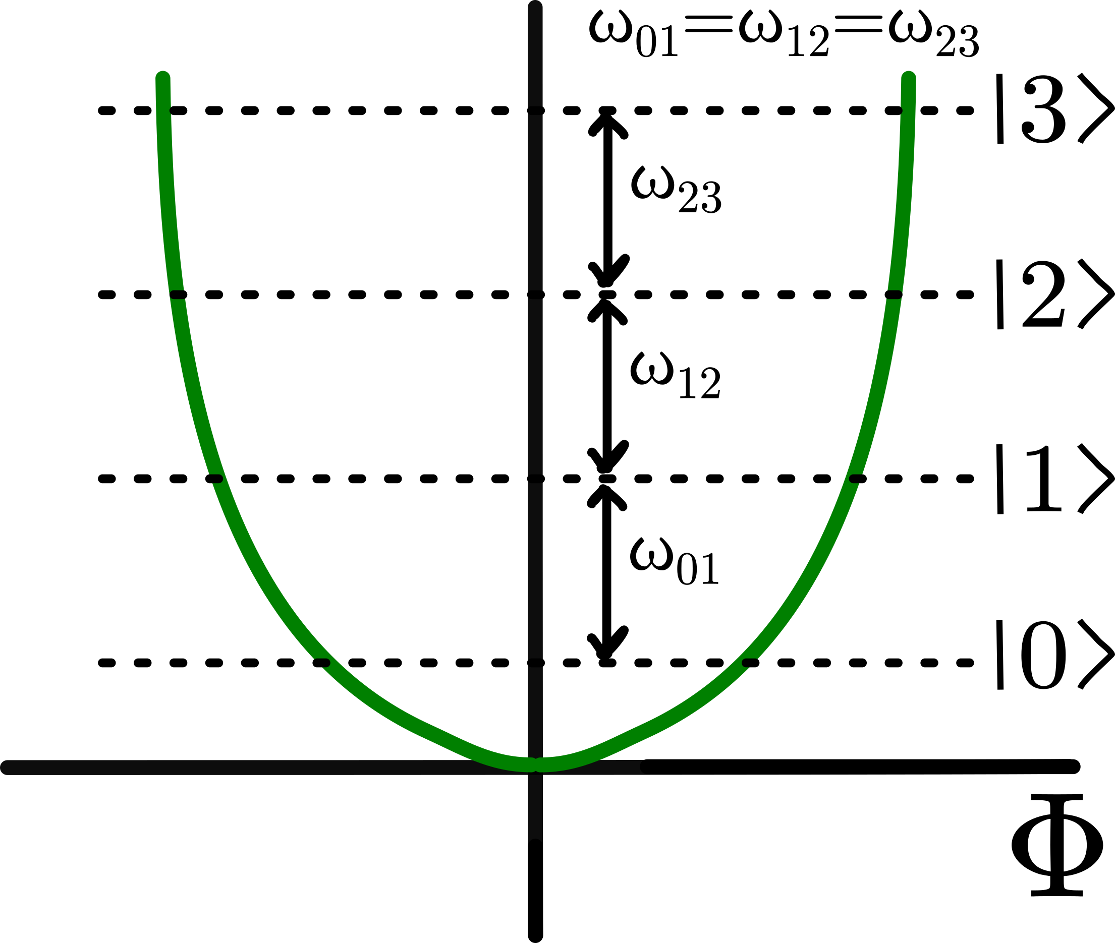
But one problem arises: Remember, we want very good controllability. We need to be able to put energy in, and be reasonably sure the qubit goes from $\ket{0}$ to $\ket{1}$, not $\ket{0}$ to $\ket{2}$. With our designed system, we can’t get that! The reason is because the ideal quantum harmonic oscillator is linear. The spaces in between $\ket{0}$, $\ket{1}$, and $\ket{2}$ are all the same in our energy diagram. Thus, the frequencies of the waves needed to transition the system from state to state are all the same. Putting in the frequency $\omega$ could excite the system from $\ket{0}$ to $\ket{1}$ or to $\ket{2}$ - this is unacceptable! We need to make the energy levels in the system non-linear (i.e., space them unevenly). The term quantum engineers use for this is anharmonocity.
We get this by substituting our inductor with something known as a Josephson junction. This is a fancy microscopic structure that A) can be made with semiconductor manufacturing methods; B) at superconducting temperatures, has non-linear quantum behavior; and C) looks almost like an inductor, but not quite. With a Josephson junction, our energy curve changes, and the distances between states become different! This means that we would need a different frequency of microwave to excite the system from $\ket{0}$ to $\ket{1}$ than for $\ket{1}$ to $\ket{2}$. We can therefore address the exact state transition we want.
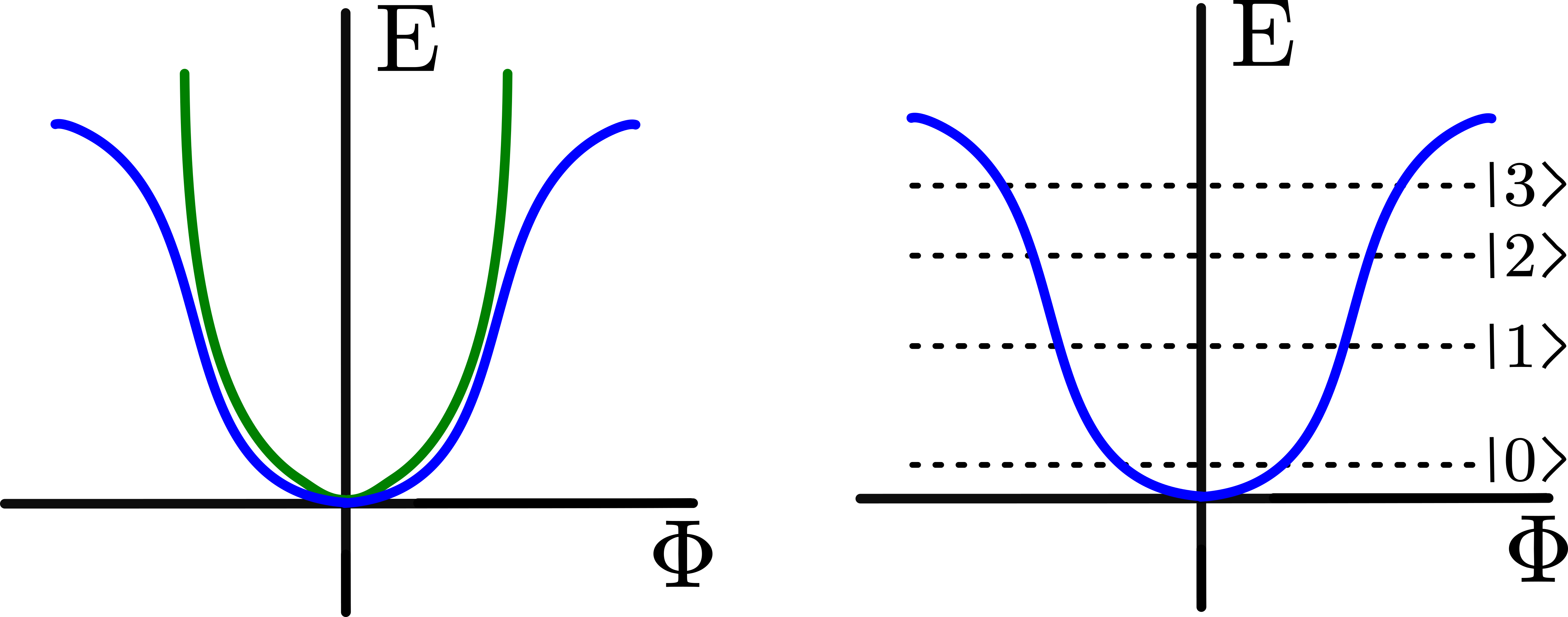
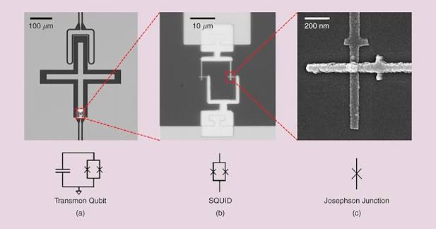
This is called the transmon superconducting qubit. There are several different kinds of superconducting qubits (fluxonium, phase, the delightfully named quantronium, etc.), but this is the one that most research groups are now pursuing, for various good reasons. As I’ve been mentioning, this is a system which can be manufactured on silicon wafers using relatively standard manufacturing principles. Some images of transmons are shown in Fig. 10. This ostensibly means that making these devices should be relatively straightforward, scalable, and repeatable! Also, the fact that these are not atomic devices, and have physical properties measured in the nanometers to millimeters, should make it easier to interact with the qubit. Functionally, a superconducting quantum computer looks like a big grid of these qubits, each which can interact with its nearest neighbors.*
However, this manufacturability has its downsides: the qubits are not exactly identical! Some of the qubits on a given chip are built faulty, and might be broken or have uneven performance (compare this to other approaches, which use particles that are definitionally identical). Even when systems are fabricated well, qubits are not necessarily identical and may have unique resonance frequencies, requiring intensive device and qubit-specific tuning.
Speaking of interaction – how do we implement gates? I’ve already told you how to do 1-qubit gates! We blast the qubit with microwaves of a specific frequency and phase, changing its state. We can calculate how much time that wave needs to completely change the qubit state from $\ket{0}$ to $\ket{1}$, and irradiate the qubit for shorter amounts of time to put it into intermediate superposition states. Furthermore, by varying the phase of the incoming microwave pulses, we can change the phase of the system, equivalent to performing gates like X, S, and T.
Two qubit gates are unfortunately more complicated. The most common way of implementing a 2-qubit gate on superconductors is to blast two adjacent qubits with an external magnetic field, changing their resonant frequencies. Depending on the state of the qubits, this process conditionally moves the qubits into a leakage state (i.e., one of the qubits is in $\ket{2}$) then back down, with a phase difference. This implements a controlled phase, or CPHASE, gate. The CPHASE gate can be easily combined with some single qubit gates to be equivalent to the more recognizable CNOT gate.
Remember that we don’t need to be able to implement every kind of single and multi-qubit gate to be able to get universal quantum computation. As long as a quantum computer has access to a universal gate set, it can always compile any program down to the gates it does have (although it might use more operations than we hoped for!).
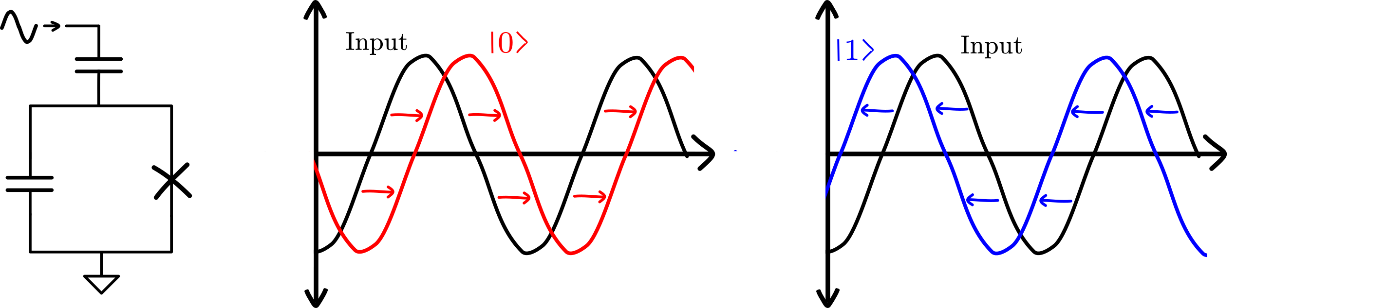
Finally, we need to be able to measure the state of the qubit. Here’s the crude, roughly correct version: inject a waveform into the qubit and measure the phase shift of the reflected signal. Because the qubit has a slightly different resonant frequency depending on its state, that phase shift should be either negative or positive, corresponding to $\ket{0}$ or $\ket{1}$. This process is called ‘dispersive readout’.
The reason why that description is not quite correct connects very directly to the challenges of superconducting qubit engineering. It turns out that readout is extremely hard to do well. The qubit is very sensitive to noise of all kinds. Measurement of the qubit can put it into a leakage state (such as $\ket{2}$) which will then propagate to neighboring qubits, ruining calculations. Thus, the readout process is carefully engineered, and all the circuits upstream must be designed to not inject any heat back into the qubit itself. This functionally looks like A) additional resonators integrated into the chip itself, which do filtering; B) amplifiers and isolation that sit in different parts of the dilution fridge. Even with these precautions, anti-leakage propagation methods must be inserted into our error correction circuits*. Oh, and by the way – all of these protections make our readout slower! It’s sort of a massive balancing act trying to optimize qubit coherence times (how long they last in a desired state); noise and leakage; and speed – all of which are critical to building a functioning quantum computer.
With regards to speed and lifetime: Superconducting qubits are much less stable than other qubit implementations. They decohere on the order of milliseconds, which implies aggressive error correction is needed to keep computations accurate until completion. This is significantly shorter than most other kinds of qubits, as we’ll see.
The flip side of this is that superconducting qubits are expected to be much faster at computing than other qubit implementations. Gates should take roughly tens of nanoseconds, and readout somewhere in the tens to hundreds of nanoseconds. This translates to operating frequencies in the MHz*, well below the multi-GHz clock speeds of conventional CPUs, but well above what trapped ion and neutral atom qubits can achieve today. This should reinforce our intuition about needing to find problems for quantum computers to solve that have very large speedups over classical computers, because doing an $O(n^2)$ computation on a quantum computer will still take much longer than an $O(n^2)$ computation on a CPU.
Let’s add another challenge to this mix: How do we even build this thing? Well, I’ve mentioned already that we can make superconducting qubits on silicon. These things look like computer chips! However, on a regular chip, we can use multiplexers, memory, and various communication protocols to interface with lots of bits at once. If you tell your CPU to add two numbers, it just needs two indices in memory and an ADD command. We unfortunately don’t have that degree of flexibility with superconducting qubits. We have lots of qubits, and need individual connections to each to be able to control them. This problem manifests in space constraints on the chip and in the dilution refrigerator, since all that control circuitry, amplifiers, and isolation take up a lot of volume too! Moreover, the more qubits you have, the greater risk that they interact with each other in ways you aren’t planning for (we call this crosstalk). And to make matters worse, it’s actually hard to make identical qubits at scale. Even successful chips often have several malfunctioning qubits which either operate with higher error rates or simply can’t be used. So far, labs have successfully scaled up to the $\sim$100s of qubits range, but breaking past that barrier will require either successful scaling using multiple interfaced chips, multiplexing on single chips*, or by some fundamental improvements that increase how many qubits can be put on one chip.
We’re not to the point where we understand multiple qubit architectures, but let’s attempt to keep track of some of the strengths and weaknesses of the superconducting qubit:
- We can make them relatively easily. That means more testing, more iterations, and more data. However, because they are human-built, they aren’t always manufactured perfectly, and qubit-specific tuning is usually required.
- We build them on a grid and can get good two qubit gate operations with their neighboring units. However, they are on a grid, and can’t be moved around!
- They’re fast, with gates approximately 100-1000x faster than other qubit architectures. They also decohere 100-1000x faster than other types of qubits! They are incredibly sensitive to noise of all kinds. They need to be kept at sub-1 Kelvin temperatures* and continuously monitored with error correction schemes.
Trapped Ions
If superconducting qubits are the 1A of most developed qubit technology, trapped ions would be 1B. This is the favored approach of many academic groups and several high-profile startups, including IonQ and the Honeywell-spinout Quantinuum. In many ways, they are the yin to superconducting’s yang: Long coherence times, high qubit interconnectivity and mobility, relatively balmy ($\sim$2-4 Kelvin) operating temperatures, and slow operations. But this isn’t to say that a trapped ion quantum computer is a simple-to-implement affair. Just like their superconducting brethren, there are significant engineering challenges to scaling these systems up.
Trapped ion quantum computers use, as their name suggests, ions as their qubits. Think back to high school chemistry class and you might remember that an ion is an atom that has a positive or negative charge due to the loss or gain of electrons. Ions are nice because they are identical and fungible (this will be a common theme among trapped ions and the next few qubit approaches). No engineering needs to go into making the qubits themselves ‘better’. They simply exist in nature! Instead, efforts go toward interfacing with and manipulating these particles. That’s where the ‘trapping’ comes in.
Ions are definitionally charged particles. Absent any sort of control, a bunch of identical atoms would all move away from each other (since alike charges repel), and we’d have no hope of interacting with them. The good news is that we can use that charged nature to our advantage and apply external electric fields to manipulate the positions of the ions. These electric fields are switched on and off extremely quickly to keep the ions in a stable position, and can be specially controlled to move the ions around.
The way this practically works is that labs and companies will use silicon chips (made with standard semiconductor processes) that have carefully designed electrodes on them. Then, ions around the system become ‘trapped’ as the electrodes start switching. The ions don’t actually get stuck onto the surface of the chip! They actually float above just above ( 50 microns) the electrode surface, in a particular zone of manipulated electric field, as shown in Fig 12.
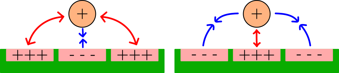
Note that we only want to trap the ions that we want to do computation with. As such, ion trapping is typically done in a controlled and supercooled vacuum ($\sim$4 K), to limit outside particles and interference with the qubits.
These ions are typically metals like calcium, barium, and ytterbium. When these elements lose one of their outer electrons, they are left with a singular electron in their outermost orbital. Outermost orbital, you ask? Again, remember high school chemistry. In an atom, electrons exist in discrete spatial bands, called orbitals. Each orbital can only be occupied by a certain number of electrons. Once a given orbital is full, electrons have to start filling the next one up. Lower orbitals have lower energies. An atom or ion in its ‘ground state’ will generally have all its electrons in their lowest available orbitals.
If an ion is perturbed with some sort of external energy though, some of its electrons can move to higher orbitals – we call this an excited state. Having only one electron in the outermost orbital means that it is simpler to analyze the ion, since most of its excited states will just involve that single electron hopping between higher energy orbitals. Hopefully you see where this is going: We can encode quantum information in these different states of the ion. The basic energy diagram for a prototypical trapped ion qubit looks something like Fig. 13.
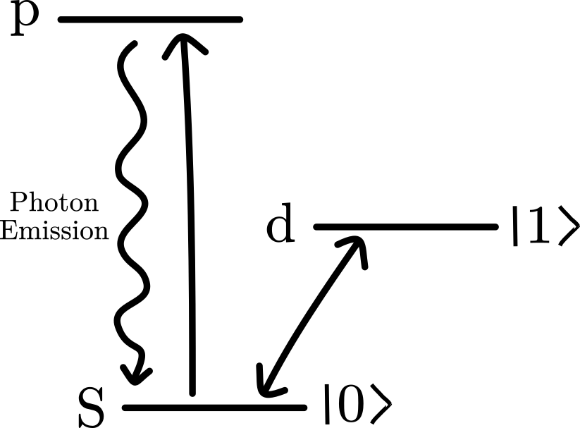
The ground state, where all electrons are in their lowest energy levels (and the highest occupied orbital is $s$), encodes $\ket{0}$. If an electron jumps to the $d$ orbital, the qubit is now in the $\ket{1}$ state. Those two levels are separated by a very well-defined amount of energy, and a laser with a specific wavelength can stimulate that transition. This should feel very similar to superconducting qubits, but note that these ions naturally have very high anharmocity! That laser only excites the $\ket{0}$/$\ket{1}$ transition, and nothing else. The time duration and phase of that laser pulse determine what kind of single-qubit gate the ion experiences. Note also that the times necessary for that laser to drive gates are on the order of milliseconds, much slower than the superconducting systems previously discussed.
To do readout, the qubit is excited with a different laser. This laser drives an electron transition from the $s$ orbital ($\ket{0}$) to the $p$ orbital. If the qubit is in $\ket{1}$, nothing happens. If the qubit is in $\ket{0}$ (or collapses to it), then it is driven to $p$, then rapidly decays back to $\ket{0}$. In that process, the qubit emits some photons (light!), which can be detected. So readout is quite straightforward: blast the qubit with a laser, then try to detect light. This does end up being practically tricky (as just about all the details of any qubit implementation tend to be), because those emitted photons might scatter everywhere, disturbing the states of all the other qubits in the system. There are various schemes that mitigate this effect.
Now this is almost correct, but real-world implementations differ slightly. What I’ve described above is called an ‘optical’ qubit, since the wavelength of light separating $\ket{0}$ and $\ket{1}$ is in the visible spectrum. The lifetime of the optical $\ket{1}$ state is fairly long, about a second. This is already miles better than superconducting qubits, but for various reasons, many of the trapped ion companies actually use a different implementation called a ‘hyperfine’ qubit.
While optical qubits operate on energy scales in the hundreds of THz*, states in a hyperfine qubit are separated by energies in the GHz, and require microwave (also known as radio frequency) pulses to drive transitions. This is because the $\ket{0}$ and $\ket{1}$ states here are encoded in two different narrowly separated energy levels of the ground state (where the outermost electron is in the s orbital), known as hyperfine levels. The advantage of these qubits is A) extremely long coherence – hours to days to weeks; and B) being able to control them using electronics rather than precisely tuned optical lasers. In most other aspects, they’re similar to optical qubits.
Just because qubit coherence is so long for ions, doesn’t mean error correction is unnecessary. These qubits may remain in the same state for a long time absent noise, but there is unavoidable noise in any quantum system. Moreover, just like in superconducting systems, the gates themselves and the readout process may introduce errors. So error correction is still vital to successful large scale computation for trapped ion systems. That being said, it’s not as critical to small scale tests, and seems to be a lower priority for most of the trapped ion players. In particular, Oxford Ionics (formerly an independent company but now an IonQ subsidiary with a unique technological approach) seems to be focusing all of its efforts on increasing gate fidelity and somewhat punting on error correction, at least for the time being. This does seem to be working, given that they have demonstrated 4 9s (99.99%) of two-qubit gate fidelity.
Speaking of two-qubit gates… trapped ion systems have a wonderfully elegant way of implementing two qubit gates. It turns out there’s a ‘hidden qubit’ lurking in the middle of this system of ions. So far, we’ve been talking about these ions as if they are isolated particles: I point my laser at one qubit, do a gate, point it at another one, and do another gate. Well, these ions are sitting in a line and interact with one another (once again, remember that particles of like charge repel each other). There are certain stable ‘modes’ of interaction or motion that can exist in this line. Think of this like standing waves on a string or spring, as shown in Fig. 14.
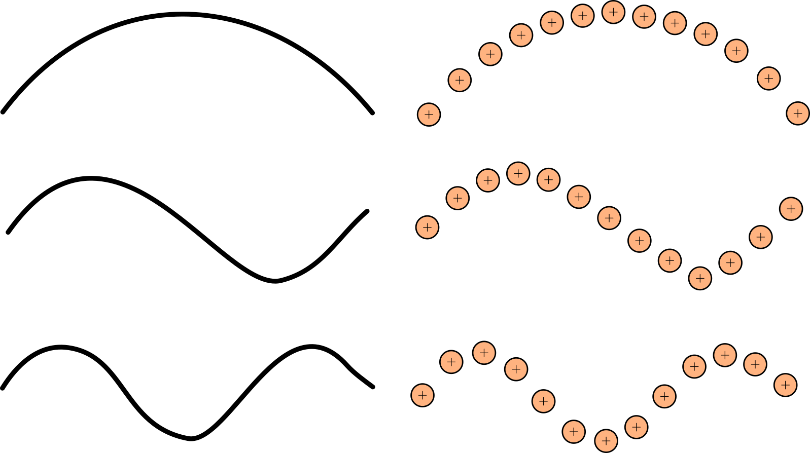
This motion is another system that behaves quantumly! Thus, we could use it as a qudit of its own (not a qubit, since there are many possible states). However, this is a shared property of groups of ions in the system, so it is practically more useful to use it as a method of sharing quantum information – i.e. performing two qubit gates.
The mechanism for this is very similar to 1-qubit gates: driving the ions with lasers. However, in two-qubit gates, these laser pulses are tuned to have additional components slightly off the wavelength they would typically use for $\ket{0}$ to $\ket{1}$ transitions. These are known as ‘sideband’ pulses. The sideband excites (or attempts to excite) the motional state of the ion system. With a red (lower energy) sideband, we could go from [qubit state $\ket{0}$, motional state $\ket{1}$], to [qubit state $\ket{1}$, motional state $\ket{0}$], as shown in Fig. 15. However, trying to excite a qubit in [qubit state $\ket{0}$, motional state $\ket{0}$] with that same laser will do nothing.
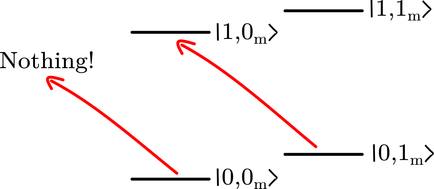
The simplest implementation of a two-qubit ionic gate relies on the asymmetry in this system: A red sideband will do nothing if the qubit is already in its lowest energy motional state. As a result, a sort of conditional logic is created by applying such laser pulses to multiple qubits, then letting them interact. Most real systems use a more complicated, but more generally applicable two-qubit gate called a Molmer-Sorenson gate. Note that this gate performs its operations natively in the X basis, rather than the Z basis, so some rotations are necessary to properly implement a CNOT.
Importantly, these multi-ion interactions have a sort of locality to them. In a chain of 100 qubits, it may be possible to make the 40th and 50th qubits entangled via a two-qubit gate, but impossible to do so with the 1st and 99th qubits. This may seem ‘bad’, but it’s already quite a bit better than superconducting qubits, who only have nearest neighbor connectivity. This interconnectivity could be made even better by making the ions mobile, as all the companies in this space plan to do. A key selling point of trapped ion systems is this ability to have greater qubit-to-qubit interactivity. This may enable easier implementation of certain algorithms and error correcting codes (think specifically of LDPC codes, which require non-nearest neighbor interactions).
This all sounds totally hunky-dory. We’ve got great fidelity and connectivity! What’s the catch? Well, laser control of these qubits is a very difficult engineering challenge, both in terms of figuring out all the multi-qubit interactions and in terms of physically building and controlling the laser systems. As a result, we really don’t want to have a line of hundreds to thousands of qubits, each with its own laser. Instead, most proposals for scalable trapped ion systems involve moving ions around from active computation zones to storage zones. See Fig. 16 for an image from Quantinuum’s newest Helios processor for an example of this: Computation gets done by fixed laser arrays pointing at the two strips, while qubits get shuttled in and out of the storage ring.
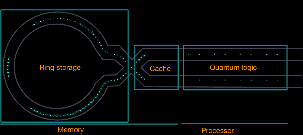
But perhaps the most important catch is timing. Transport takes time, currently on the order of tens of milliseconds. In addition, after every transport, ions must be cooled down, which also adds tens of milliseconds. After all is said and done, gate operations can be performed on the order of milliseconds as well. Functional clock speeds may then be in the kHz range, significantly slower than superconducting systems (and comparitively glacial to a normal classical processor). Clearly, optimizing all aspects of the system for higher speed will be necessary to get to scalable quantum computing. It’s unlikely that trapped ion systems will ever be as fast as superconducting ones, but there is progress left to be made.
Next problem: Controlling lots of lasers is really hard and very bulky! Different groups have different approaches to solving this problem: Lots of folks are betting on integrated photonics – essentially building laser optics into the semiconductors themselves. This is still a nascent approach, but could drastically reduce the complexity of building these systems. The previously mentioned Oxford Ionics is taking a very orthogonal tack, and choosing to minimize laser usage altogether. Their goal is to use integrated optics to do state initialization and measurement, but use electric fields to perform gate operations. It’s far too early to tell which approach, if any, will win.
The long-term vision for trapped ion systems is to have multiple chips, each with hundreds of ions, networked together. This is ultimately the most feasible way to achieve scalability to systems with millions of qubits. Individual chips would be able to generate entangled photons via ion/ion interactions, then send those photons (with quantum information embedded in them) to interconnected chips via fiber optic cables. Trapped ion systems are far from this stage of development, but it is a critical piece of their future development roadmap.
Phew! Another one bites the dust. Once again, let’s summarize some of the high-level tradeoffs of this modality:
- Advantages: Trapped ions are totally identical and extremely controllable. They are quite resistant to noise, and extremely stable and long lived. They have good inter-qubit connectivity, which enables lots of great things from a computation perspective.
- Disadvantages: They are extremely slow, and scaling to larger qubit-count systems will require huge amounts of infrastructure and difficult engineering.
Neutral Atoms
Much of the following will rhyme with the trapped ion situation. Atoms are extremely similar to trapped ions, mostly because ions are just atoms with an electron removed or added. These systems encode qubits in the same way, between different energy states of the atom (where its electrons are in different orbitals). This leads to similarly long coherence times. In general, the gate operations are similar too. And just like trapped ions, atoms can be shuttled around to enable non-local entanglement or storage.
Perhaps it’s more edifying to focus on the differences. Neutral atoms are definitionally neutral. That’s both good and bad: trapped ion systems have to do active control to contain their charged particles, because without it, those like charges would repel. But that electric field control lends itself nicely to implementing chips with integrated electrodes that can trap and shuttle ions around. On the other hand, atoms are happy to be near each other, and most quantum computer proposals & demonstrations in this space end up implementing systems as a large rectangular grid of atoms. As for containing and manipulating those atoms, the solution is lasers! We’ve glossed over it before, but lasers are used for cooling in both trapped ions and neutral atom systems (see box below). We add one more level of laser application for trapped ions, known as ‘optical tweezers’.
These tweezers are focused beams of laser light. At their focal points, there is a location of low energy where the atoms will naturally sit. These beams can pick atoms up and move them around. Controlling those beams at scale is a unsurprisingly difficult problem; the most common approach relies on a device called an acoustic optical deflector (AOD). An AOD is a special kind of crystal that can break a single incident laser into multiple output beams, each adjusted by a certain angle, all controlled by an input acoustic signal. It’s incredibly cool engineering!
This control mechanism is advantageous for scaling on both fronts: We can have arrays of many atoms that can be moved around (potentially in bulk!) and it is not impossibly difficult to generate lots of tweezers that do the moving. But because these atoms are not ‘trapped’, they do happen to have a problem getting lost in the middle of operations. As such, a fully realized atom-based computer likely needs to be able to actively replace atoms in its system.
Laser Cooling
In our popular imagination, lasers lay somewhere between death rays and fun cat toys. In both cases, the laser shoots out light and hits something. In the weapon application, that laser has a lot of energy and heats its target up, perhaps in explosive fashion. In many neutral atom quantum computing systems, not only do lasers hold the qubit in place, they actually cool the atom down all the way to several micro-Kelvin (this technique is also used in trapped ion systems too!). This is pretty unintuitive!
The primary laser cooling process used is known as ‘Doppler cooling’. To understand how it works, we need to know a few prerequisite facts:
- Heat in a system is equivalent to the motion of the particles in the system. If particles are moving more slowly, that system is cooler.
- An atom/ion will absorb an incoming photon if the photon is of a particular frequency. If a photon is absorbed, the atom/ion will go into an excited state, then emit another photon when it drops back into its ground state.
- The Doppler effect explains why an observer can perceive different frequencies depending on the relative motion of the observer and the incident particle/wave. The classic example is listening to a police siren as a cop car drives by: The wail is higher pitched (higher frequency) as the car drives toward you, and lower pitched as it drives away from you.
Put these concepts together and you get laser cooling: Tune a laser to be slightly lower than the excitation frequency of the atoms/ions, and point it at the bunch of particles you want to cool. Then, the particles moving toward the laser actually experience photons at their excitation frequency (because of the Doppler effect), while particles moving in any other directions will be unaffected. So this subset of particles absorbs photons, which lessens their momentum. Crucially, when they later emit photons, they do so in a random direction, so on average, whatever momentum that the emission contributes is less than the initial slow-down from the absorption. Over time, this cools down our mass of particles down to the ‘Doppler limit’, which is good enough for many quantum applications. There are advanced techniques that can get down even lower. Cool!
Another difference relates to the implementation of two-qubit gates. Neutral atom implementations rely on something called ‘Rydberg states’. When an atom is in a Rydberg state (also called a Rydberg atom), its outermost electron is in a much higher orbital, farther away from the nucleus. These Rydberg atoms are more prone to interactions with other atoms, and it is these interactions which enable two-qubit gates. The standard CNOT gate elevates one qubit to a Rydberg state, and it conditionally interacts with another qubit, depending on the second’s state (the interested reader may want to look up this process, known as a Rydberg blockade). In general, this is a pretty fast operation, occurring under a microsecond. This is significantly faster than two-qubit operations in a trapped ion computer.
One very exciting quality of neutral atoms is that it may be possible to perform gate operations en masse – i.e. making large blocks of atoms experience the same gates. While it doesn’t seem like this has been implemented in a commercial quantum computing system yet, this quality has the ability to further improve neutral atom-based approaches’ scalability.
There’s a subtle distinction between different implementations of these schemes. Some have a more static grid of qubits and can implement gates between non-local qubits (of course, with some limitation in range). However, most schemes have segmented regions for two-qubit operations, readout, and storage. This is easier in some regards, but does require more qubit transport. There’s always a tradeoff!
The different atomic startups differ mostly in how the encode their qubits. The most popular choice is in the hyperfine states of rubidium atoms, although Atom Computing uses nuclear spin states of strontium, and Infleqtion uses two different kinds of atoms (a ‘dual species’ approach). Some of the startups (and parts of academia) are also interested in building `quantum simulators' (which are akin to analog computers) with their atoms. This is a more natural fit for atom based systems because even today, they have lots of controllability over atom positioning. As such, you could imagine (and if you have the right equipment, actually conduct) experiments wherein atoms are arranged in particular 2D or 3D patterns, then allowed to evolve over time. Some measurement of the system’s properties could then reveal something about the problem you are attempting to solve.
Let’s do our review then: Neutral atoms have long coherence times and have fundamental advantages in system scaling, especially at the 100-1000 qubit level. Their gate operations are pretty fast too! Perhaps their biggest disadvantage now is that the approach simply isn’t mature enough. There are very difficult control problems, especially at high qubit counts, that need to be dealt with in these systems. Experimental data has shown very similar learning curves for two-qubit gate fidelity for superconducting, trapped ion, and neutral atom experiments. However, since neutral atom experiments started later than the other technologies, their gate fidelities still lag behind! Time will tell if these companies catch up, or get left behind.
Photonic
You may be seeing a pattern: Find (or engineer) a system with quantized energy states, isolate it from its environment as much as necessary, use specially tuned pulses of energy to transition it from state to state, and a quantum computer is created! Unfortunately, photonic quantum computers render this hard-earned intuition virtually useless. To make matters worse, photonic approaches not only differ radically from their superconducting/ion/atom brethren, they also have a great deal of internal variance – the approaches of the various photonic companies are not necessarily simpatico. All of this is because photons are so fundamentally different than the other qubit building blocks we’ve covered. They have very unique strengths and shortcomings that influence how a computer utilizing them should work.
First of all, photons are extremely mobile. Superconducting qubits are big and stationary; atoms will rest in place; even ions can be trapped and manipulated. Photons literally never stop moving. From the moment they are generated to the moment they are destroyed, they are moving at the speed of light! This is sort of exciting in some sense – we’ve talked a little bit about the necessity for quantum communication between different processing units, and something that can move while having quantum properties could be very useful. It’s also, on another level, incredibly inconvenient for computation. A quantum computer has to make decisions on the fly about what gates to apply to a system (quintessentially, this is part of error correction). That’s all well and good when your qubits are always in the same spot, but practically much harder when they are flying through the system at $3*10^8$ meters per second.
That is, if they even are in your system. Photons are extremely mobile, to the point where at any moment they may just… get lost. Photon loss is an intrinsic part of any optical system and strongly constrains these types of quantum computers.
Finally, for better and for worse, photons don’t like to interact with other things. This makes them extremely resilient to noise and decoherence, to the point where these systems may be able to operate at room temperature. It also makes them very hard to force into two-qubit interactions. The standard way to implement a two-qubit photonic gate has a roughly 50% chance of failing in theory, let alone in practice! That’s obviously miles away from the previously discussed approaches, which have had measured two-qubit gate fidelities with multiple 9’s of fidelity.
Let’s establish some physical intuition before we start getting too theoretical though. Photons are light, and light can be moved around and manipulated using linear optical components. These optics can be standalone, discrete objects or (as is the plan of all the companies in this space) integrated onto silicon chips. Something generates the photons, it flows through the chip on waveguides and hits various optical components, then gets measured by a photodetector at the end. There are two primary kinds of linear optical components: phase shifters and beam splitters. A phase shifter does exactly what it says it does – takes the input photon(s) and adjusts its phase. A beam splitter takes an input, and splits it into two output beams. If a single photon enters a beam splitter, it will go down one path with a certain probability (which can be tuned).
It’s not intuitive to see how those building blocks can be used to build a quantum computer. But in 2001, Knill, Laflamme, and Millburne came up with their KLM scheme, which was the first real, although impractical, photonic proposal. It’s not quite how things are being developed now, but it is intellectually quite useful to think through this model first.
Their proposed approach is what is known as a ‘dual rail’ scheme, wherein a single qubit is represented by a photon traversing two optical paths. If the photon is measured on one path, that’s a $\ket{0}$, if on the other, a $\ket{1}$. Single qubit gates can be implemented via phase shifters (changing phase, duh) and by bringing the two rails close together (which implements gates acting on the computational basis, since with some probability photons will jump over to the other rail). A trivially simple path, shown below, could easily implement a qubit being subjected to several single qubit gates, then being measured.
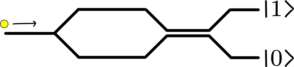
These single qubit gates can be made to be reconfigurable via ‘thermo-optics.’ Essentially, heat up the waveguide, and its properties change. Hence, gates can be re-programmable in a more general chip, akin to a conventional computer. Thermo-optics are problematic since heat A) spreads between different gates, causing correlated errors; and B) takes time to… heat up, limiting bandwidth. That’s why several of the leading photonic startups are investigating electro-optic schemes, wherein gate properties can be modified with fast-acting electric signals. PsiQuantum in particular seems to be at the cutting edge of this.
The tricky thing is how to implement a two-qubit gate. KLM’s proposed a specific scheme (now superseded by better approaches) that involved several beamsplitters interacting between two qubits and some ancillas, followed by measurement. The details aren’t terribly important, but there is one very big caveat with their implementation: it is non-deterministic. That is to say, any two-qubit gate was not guaranteed to work. Their proposal only had a 25% chance of succeeding (although that probability could be boosted with the addition of ancilla photons and additional work). I want to emphasize this. If a two-qubit gate has a 95% chance of succeeding and a 5% chance of destroying both qubits, after 1000 gates (a relatively small quantum circuit), the system has approximately a 1 in $10^{23}$ chance of getting an output. So this non-determinism is really a tremendous problem for large-scale computation! It’s nigh impossible to get this approach to scale. You’d have to run computations repeatedly until you got a result for unfeasibly long times.
Nevertheless, the KLM proposal was a very important milestone for the field and stimulated a lot of incremental improvements and novel development. Better schemes for two-qubit gates were developed, and much attention was spent on photon generation. It is in fact extremely difficult to generate high quality, single photons on demand. As we will discuss later, this is a rate-limiting factor for several of the current leading approaches in the field. Bits of the KLM scheme end up even in the more advanced, current approaches to quantum computing, and implementing a KLM-style processor is an attractive intermediate proof of concept that several startups have built.
The big ‘a-ha’ moment in the field came from the concept of ‘cluster states’ and measurement based quantum computing (MBQC). Remember way back in Chapter 1 when I told you that circuit-based quantum computing isn’t the end-all-be-all of the field? Well, that chicken has come home to roost. The photonic people realized that if you have a system where it is really hard to do two-qubit gates, it might behoove you to pick a style of computation where you try to minimize the use of those gates. Thus, the selection of MBQC.
MBQC is not exclusive to photonic based computing, but it is very well-suited to this modality. The fundamental idea is that the system prepares a large, entangled, multidimensional state, called a cluster state. That state then undergoes a series of conditional measurements in varying bases*. These measurements (which have a kind of logic built in) actually do the computation.
Conceptually, it is a very different way of thinking about doing computation, but it is mathematically equivalent to the circuit-based model: anything that can be done with gates, can be implemented with MBQC. As a result, you can still think about algorithms for photonic quantum computing in terms of gates, but their compiled implementation will be very different.
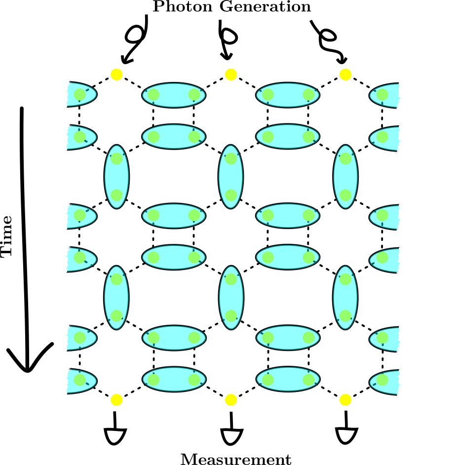
The MBQC model is useful for photons for a few reasons:
- You do the really lossy two-qubit gates and entanglement first, and can potentially just post-select the photons in the correct state from the failed goes.
- That cluster state is multi-dimensional, and one of those dimensions can be time! So if you can generate a continuous stream of photons, delay some of them, then entangle them with the next ‘generation’, that sufficiently implements such a state. So a very large cluster state can be generated over time, which is very suitable for an implementation where qubits are constantly getting destroyed. Moreover, that cluster state can be imperfect, with failed operations or missing qubits, and computation can still be done.
- The lifetime of a qubit is relatively short: It gets created, entangled, then measured. That’s it! That reduces the opportunities for the photon to get lost or to have some sort of error in a gate.
Somewhat important asterisk here: PsiQuantum, one of the leading photonic companies, has their own special flavor of MBQC they call ‘fusion based quantum computing’ (FBQC). FBQC is structurally very similar to MBQC, but has some additional tradeoffs. The MBQC method requires a large cluster state to begin with, which might require a lot of entanglement and happen with lower probability. The FBQC folks say look, what if we create simpler, smaller entangled states, then do a more complicated measurement scheme after the fact (with their destructive ‘fusion’ measurements). That lets them build a more complicated full calculation without having to make extremely large, entangled cluster states. The trouble is that the measurement scheme (consisting of fusion operations, hence FBQC), is non-deterministic. So they probably will need more resources, comparatively, to implement that scheme.
We’ve covered most of the system so far: we know how the systems do computation, how the qubits are encoded, and how gates and measurement are implemented. There’s one more important detail – how do we make these photons in the first place? It’s easy to make light: we can do that with lasers no problem. But these schemes require a very particular kind of light – identical single photons! Most light sources make lots and lots of photons at a time, often not typically identical ones. We want very high purity and high precision. There are a few varying approaches of doing this, but none are quite at high scalability yet. PsiQuantum uses these things called spontaneous four wave mixers (SFWM), that do pretty well, but yet again, they are probabilistic. That’s problematic, because we’d like all of our photons to be ready to go at the same time, so that we can entangle them and inject them into the system. Their plan is to multiplex lots of these units with lots of switches and delay lines to get things into the right state. That’s somewhat plausible, but going to be difficult to implement. Quandela, another startup, takes a different tack: They use quantum dots* to generate photons. The quantum dots, when excited with a laser, emit single photons with high precision. The trouble with this approach is that it’s really hard to make identical quantum dots en masse. So in both cases, photon generation is the limiting factor – and you need lots of photons!
Yet again, there’s another startup with distinct approach. Xanadu, a Canadian startup, thinks single photons are too hard to implement at scale. So instead, they use lots of photons, in the form of laser pulses. These pulses are put into what are known as ‘squeezed vacuum states’. Unfortunately while these squeezed states can be used to implement much of quantum computation, they are not universal; as a result Xanadu also has to create a special state (called a GKP qubit) probabilistically. Their computational approach bakes in the fact that they won’t have only GKPs, but otherwise proceeds more or less like the above MBQC methods.
And so we’re left with our photonic quantum computer: Blazingly fast, resistant to decoherence, (mostly*) room temperature, but hard to scale and control!
Other approaches
The above four platforms are by no means the only ways people have tried to (or are trying to) implement quantum computers. In fact, the list of possible qubit candidates is too long for me to cover. I’m choosing to highlight a few other high profile (or high potential) alternative platforms below.
Quantum Annealers
Quantum annealing is a strange beast. It’s kind of a technology platform and kind of a method of computation. It’s frankly ill-defined theoretically, so perhaps it’s best to just describe the systems that perform it, known as annealers. After initial academic proposals, the company D-Wave was founded to develop commercial quantum annealers in 1999 – well ahead of any other dedicated quantum computing startups! For all intents and purposes, D-Wave is the quantum annealing field all by itself. For over 20 years, they’ve pressed forward with the idea that their limited version of quantum computing could get to market faster, demonstrate value, and win over customers.
The D-Wave system consists of a grid of superconducting ‘flux’ qubits (the newest version of their annealer has about 5000 of them). These are different than the transmon qubits we learned about earlier – they have a potential diagram that can form two different energy wells, shown in Fig. 19. One of these energy wells represents binary 1, and the other represents binary 0. The system is slowly transitioned from something that looks more like a harmonic oscillator (like the transmon qubit) to this binary well system.
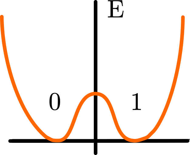
On the grid, each qubit has some physical connections to neighboring qubits, called couplers. These couplers are programmable, and can set different relationships between their qubit pairs. The qubits and the couplers are initialized to some state that represents a problem of interest (think of this as some sort of generic optimization problem). The problem is encoded in a way that the lowest energy state of the annealer corresponds to the solution of the problem. The system is evolved over time, with the goal of slowly getting the system to that minimum energy state. Because the system is quantum, it can hopefully get out of local minima that would trap classical approaches (like in Fig. 20).
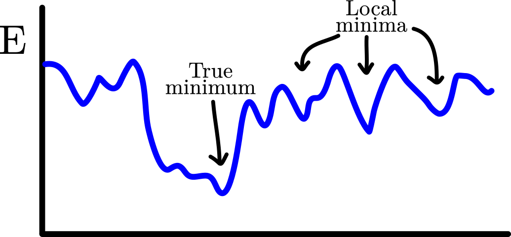
This process is closely related to the concept of adiabatic quantum computing, where a system is initialized into a starting Hamiltonian, slowly evolved over time with the goal of getting to some sort of final/solution energy state. Adiabatic quantum computing is a fully universal quantum computing paradigm, and is mathematically equivalent to the gate-based model. However, truly adiabatic computing is hard to do! It requires very low temperatures (lower than even most superconducting systems operate at) and could require very long evolutions of state to get to an answer (which could push well past the decoherence times of currently available hardware). The quantum annealing concept essentially implements a version of adiabatic computing with limited scope. It makes less strict requirements regarding temperature & state evolution, and can only operate with particular kinds of Hamiltonians (those flux qubits have to end up in a binary state).
D-Wave’s story is appealing in some ways: Limit flexibility in problem solving, but simplify the hardware requirements and make things feasible faster. And they have gotten to high qubit counts (thousands!) and attracted lots of funding in the process. However, the quantum annealing method is fundamentally a heuristic one, and it’s completely unproven if it can reach an exponential speedup in any sort of practical optimization problem. D-Wave has done some simulations of ‘spin glasses’ which may be intractable classically, but these experiments seem to lack practical utility as well. As a result, the quantum annealing approach has totally fallen out of favor, especially as gate-based qubit platforms reach greater maturity, and the prospect of fault-tolerant computation seems possible.
Perhaps the most telling sign of the times is D-Wave’s acquisition of Quantum Circuits Inc. (QCI) in early 2026. QCI is a company building superconducting qubits for error-corrected, gate-based computation. D-Wave says they are going to push forward with both approaches, but it’s clear that quantum annealing is destined to be an also-ran.
Topological
I need to make a confession here: I am totally out of my intellectual depth when it comes to topological qubits. In my defense, I’m in good company with my confusion. Every layman’s explanation of topological qubits ends up saying something like the following:
Topological qubits are a proposed qubit implementation that encodes quantum information in the structure/shape of the system that composes the qubit. As a result, these qubits are expected to be much more resilient to noise than other approaches.
Which frankly, tells you absolutely nothing. There is then some diagram that looks like a bunch of pieces of string hanging from holes, like in Fig. 21.
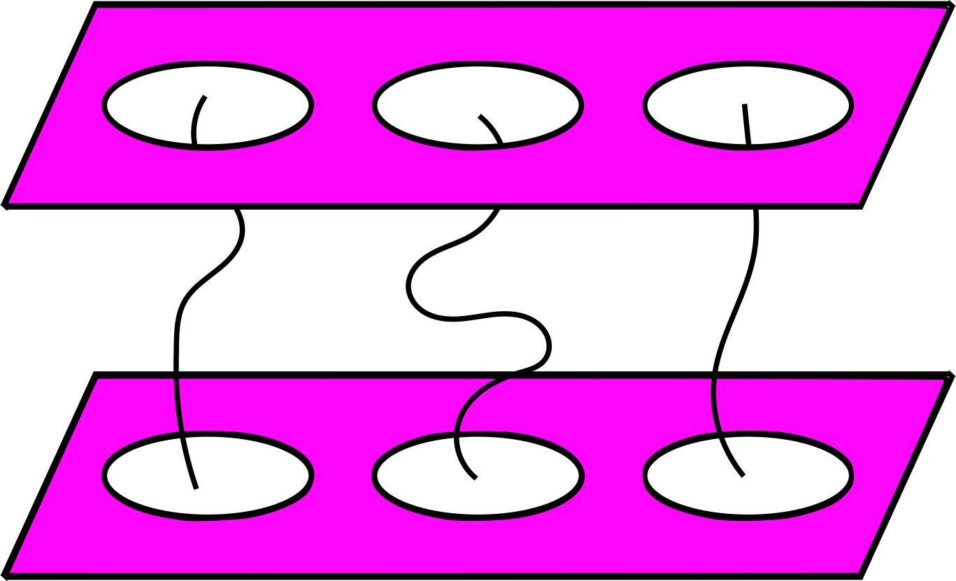
Apparently, a topological qubit is just like a piece of string. Noise might wiggle that string around, or create a loop, but it’s not going to change what holes the string comes out from or goes into. Thus, noise doesn’t affect the quantum state! Or at least, it affects it less?
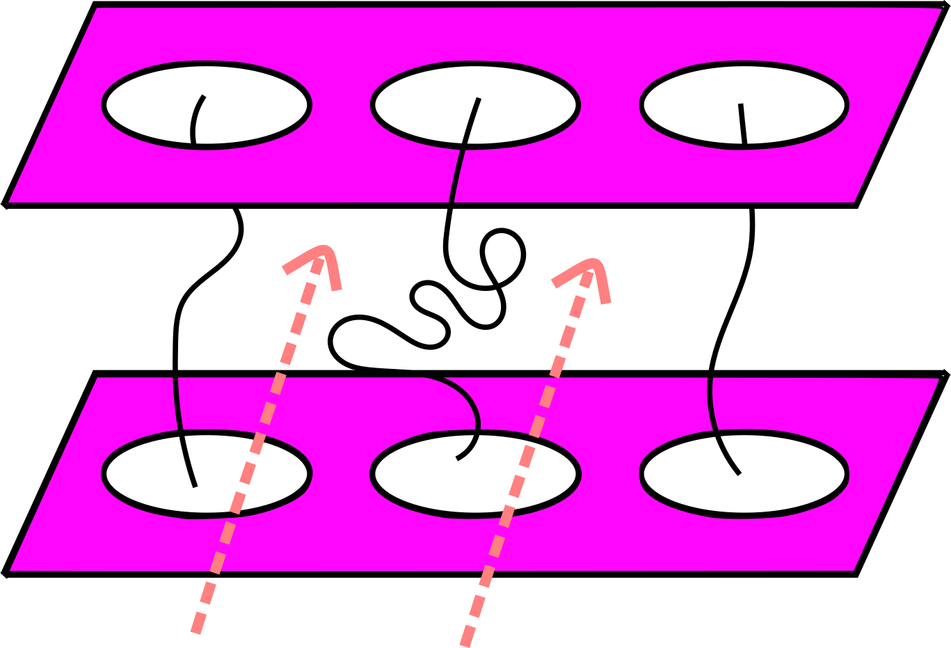
These qubits can be implemented via something called a Majorana quasi-particle, which is a special quantum particle (never actually observed, only theorized!) that has this topological property. Since we’ve never seen one of these Majoranas, we instead have to make one with semiconductors, akin to how we make transmon superconducting qubits.
In 2025, Microsoft announced to much fanfare that they had successfully created this quasi-particle, or at least that they had created something that behaved in the way that such a quasi-particle would. The paper was accompanied by a huge PR blitz, heralding the arrival of a quantum future led by our overlords at Microsoft. Unfortunately, the academic community immediately began pushing back against both the extreme claims made by the press releases and the actual data in the paper. Like I said, I can’t really make heads or tails out of the actual physics here, but there’s enough smoke in the air to make me reasonably convinced of a fire: Some of the co-authors on a prior 2021 paper asked to be taken off and several claims of data manipulation were made. Almost a year after the initial hullabaloo, Microsoft actually published a new set of results - which of course were met with another round of skepticism.
My opinion about topological qubits, which I suggest you adopt, is to not worry too much about them.
Silicon Spin
In contrast to the previous two approaches, silicon spin qubits are not necessarily fated to be an intellectual dead-end or technical boondoggle. Rather, they are an up-and-coming qubit modality with appealing characteristics and great promise!
Here’s the short story: It’s appealing to encode qubits in the magnetic spins of electrons, because it’s a naturally binary quantum system (electrons are either spin up or spin down). This does necessitate capturing and controlling single electrons, a non-trivial task. The solution is to use quantum dots, which are sort of like artificial macroscopic atoms. Each quantum dot can be controlled to confine a single electron, convenient for quantum computation. The electrons can then be manipulated through microwave radiation (just like superconducting systems) or voltage pulses on the chip. Quantum dots can be manufactured in a variety of substrates, but the most suitable medium seems to be silicon, in which A) electrons can remain coherent for relatively long amounts of time; B) be manufactured via standard semiconductor processes. Add in fast gate operations (on the same timescale as superconducting qubit platforms), and you’ve got a very attractive technology for scalable quantum computation.
What’s the catch? Well, these spin qubits are simply a less mature technology. Qubit counts are hovering around single digits today, and gate fidelities are not yet up to snuff. Manufacturing is tricky, due to high precision and tolerance needed to successfully make the quantum dots (and if the process isn’t quite right, then the qubits may have significant and problematic variation). If these problems can be addressed though, spin qubits could become a dominant qubit modality in the future! This approach is being pursued by several startups as well as American semiconductor giant Intel.
System Engineering
We now know how to build qubits, and maybe a little bit about how to enclose and control them (cryogenics, vacuums, RF fields, lasers, etc.). But in the same way that having some transistors does not make a computer, having some qubits does not make a quantum computer. There’s a system that needs to be built around the qubits to make them into something that can do computation! Let’s walk through some of these non-quantum components, starting at the user:
- Compiler: A quantum programmer is thinking in some sort of algorithm, and is choosing to implement that in some sort of high level way. After all, if computers can’t hope to simulate the states of a hundred qubits, there’s no way for a person to hold those states in their mind! So the programmer has some sort of programming language, and some sort of compiler translates those instructions into actual qubit gates. There might be multiple layers of this, where a platform agnostic compiler makes generic gates, and then a platform-specific compiler translates those generic gates into what is feasible to implement on a given piece of hardware.
- Calibration & Monitoring: This is all very dependent on the qubit modality in question, but in general there needs to be some sort of automated supervisory system for the quantum computer. This system might be automatically calibrating superconducting qubits or checking if atoms have leaked out of their optical traps, then mitigating these issues.
- Gate Control: Again, platform dependent. In general, a system must generate lots of high frequency laser, microwave, or voltage pulses with high precision, often at the same time. This is no trivial problem, and in some cases must be coupled with lots of isolation & cryogenics to reduce noise.
- Integration with classical computing: This is important on two fronts.
- First, many algorithms are hybrid quantum/classical. While the quantum algorithm is running, the system may need to do classical computation, or vice versa.
- Second and more crucially, error correction generally necessitates mid-circuit measurements and feed-forward operations, where future gate operations depend on the results of stabilizer measurements. Especially in superconducting systems, this may require extremely low latency connections and logic, implemented on an FPGA, GPU, or other specialized chip. This is tricky to actually implement, and we’ll likely see much innovation in this space moving forward.
Another axis for system integration (and seems to be the topic du jour), is the heterogeneous combination of different qubit architectures. In many ways, this is a pretty reasonable idea. Superconducting qubits can do lots of operations fast, but are bad at long term stability. Ion or atom based platforms sit on the other side of the spectrum, and may be suitable for longer term storage or some type of ‘quantum memory’. If you integrate both on a single system, maybe you can get the advantages of each. The important caveat is that system complexity will increase significantly, and communicating quantum information between different qubit modalities is a very difficult engineering problem. Nevertheless, there’s been significant buzz around this concept, with Google branching out into neutral atom approaches, funding programs being announced for the concept, and startups announcing plans for heterogeneous architectures.
So now you know how to build a quantum computer. What comes next?
References
- Victor V. Albert and Philippe Faist, “The Error Correction Zoo,” 2026, accessed April 19, 2026, https://errorcorrectionzoo.org/list/quantum transversal.
- Pedro Sales Rodriguez et al., “Experimental demonstration of logical magic state distillation,” Nature 645, no. 8081 (September 2025): 620–625, issn: 1476-4687, accessed April 19, 2026, https://doi.org/10.1038/s41586-025-09367-3, https://www.nature.com/articles/s41586-025- 09367- 3.
- Craig Gidney, Noah Shutty, and Cody Jones, “Magic state cultivation: growing T states as cheap as CNOT gates,” arXiv.org, September 26, 2024, accessed April 19, 2026, https: //arxiv.org/abs/2409.17595v1.
- N. Lacroix et al., “Scaling and logic in the colour code on a superconducting quantum pro- cessor,” Nature 645, no. 8081 (September 2025): 614–619, issn: 1476-4687, accessed April 19, 2026, https://doi.org/10.1038/s41586-025-09061-4, https://www.nature.com/articles/s41586- 025- 09061- 4.
- Rajeev Acharya et al., “Quantum error correction below the surface code threshold,” Nature 638, no. 8052 (February 2025): 920–926, issn: 1476-4687, accessed April 19, 2026, https: //doi.org/10.1038/s41586-024-08449-y, https://www.nature.com/articles/s41586-024-08449- y.
- Craig Gidney, “Quantum Error Correction goes FOOM,” accessed May 28, 2026, https:// algassert.com/post/2503.
- Xavier Waintal, “The Quantum House Of Cards,” Proceedings of the National Academy of Sciences 121, no. 1 (January 2, 2024): e2313269120, issn: 0027-8424, 1091-6490, accessed April 28, 2026, https://doi.org/10.1073/pnas.2313269120, arXiv: 2312.17570[quant-ph], http://arxiv.org/abs/2312.17570.
- Gil Kalai, The Argument against Quantum Computers, arXiv:1908.02499, August 7, 2019, accessed October 21, 2025, https://doi.org/10.48550/arXiv.1908.02499, arXiv: 1908.02499[qu ant-ph], http://arxiv.org/abs/1908.02499.
- Thomas Roth, Ruichao Ma, and Weng Chew, “The Transmon Qubit for Electromagnetics Engineers: An introduction — IEEE Journals & Magazine — IEEE Xplore,” June 2022, accessed May 16, 2026, https://ieeexplore.ieee.org/document/9789946.
- Gavin S. Hartnett et al., Fast, accurate, high-resolution simulation of large-scale Fermi-Hubbard models on a digital quantum processor, 2026, arXiv: 2605.04025 [quant-ph], https://arxiv. org/abs/2605.04025.
- R. Acharya et al., “Multiplexed superconducting qubit control at millikelvin temperatures with a low-power cryo-CMOS multiplexer,” Nature Electronics 6, no. 11 (November 2023): 900–909, issn: 2520-1131, accessed May 6, 2026, https://doi.org/10.1038/s41928-023-01033-8, https://www.nature.com/articles/s41928-023-01033-8.
- A. C. Hughes et al., Trapped-ion two-qubit gates with ¿99.99% fidelity without ground-state cooling, arXiv:2510.17286, October 20, 2025, accessed February 19, 2026, https://doi.org/10. 48550/arXiv.2510.17286, arXiv: 2510.17286[quant-ph], http://arxiv.org/abs/2510.17286.
- C Monroe, “Primer on Mølmer-Sørensen Gates in Trapped Ions.”
- Anthony Ransford et al., Helios: A 98-qubit trapped-ion quantum computer, arXiv:2511.05465, November 7, 2025, accessed January 9, 2026, https://doi.org/10.48550/arXiv.2511.05465, arXiv: 2511.05465[quant-ph], http://arxiv.org/abs/2511.05465.
- Carmelo Mordini et al., “Multizone Trapped-Ion Qubit Control in an Integrated Photonics QCCD Device,” Physical Review X 15, no. 1 (February 24, 2025): 011040, issn: 2160-3308, accessed May 6, 2026, https://doi.org/10.1103/PhysRevX.15.011040, https://link.aps.org/ doi/10.1103/PhysRevX.15.011040.
- C. M. L ̈oschnauer et al., Scalable, high-fidelity all-electronic control of trapped-ion qubits, arXiv:2407.07694, July 10, 2024, accessed October 21, 2025, https://doi.org/10.48550/arXiv. 2407.07694, arXiv: 2407.07694[quant-ph], http://arxiv.org/abs/2407.07694.
- Kenneth R Brown, Jungsang Kim, and Christopher Monroe, “Co-designing a scalable quantum computer with trapped atomic ions,” npj Quantum Information 2, no. 1 (November 8, 2016): 16034, issn: 2056-6387, accessed February 16, 2026, https://doi.org/10.1038/npjqi.2016.34, https://www.nature.com/articles/npjqi201634.
- Dolev Bluvstein et al., “A fault-tolerant neutral-atom architecture for universal quantum computation,” Nature 649, no. 8095 (January 2026): 39–46, issn: 1476-4687, accessed May 9, 2026, https://doi.org/10.1038/s41586-025-09848-5, https://www.nature.com/articles/s41586- 025- 09848- 5.
- Yiyi Li et al., Fast, continuous and coherent atom replacement in a neutral atom qubit array, arXiv:2506.15633, June 18, 2025, accessed December 30, 2025, https://doi.org/10.48550/arXiv. 2506.15633, arXiv: 2506.15633[quant-ph], http://arxiv.org/abs/2506.15633.
- M. Saffman, Quantum computing with atomic qubit arrays: confronting the cost of connectivity, arXiv:2505.11218, November 9, 2025, accessed March 6, 2026, https://doi.org/10.48550/arXiv. 2505.11218, arXiv: 2505.11218[quant-ph], http://arxiv.org/abs/2505.11218.
- Simon J. Evered et al., “High-fidelity parallel entangling gates on a neutral-atom quantum computer,” Nature 622, no. 7982 (October 2023): 268–272, issn: 1476-4687, accessed March 6, 2026, https://doi.org/10.1038/s41586-023-06481-y, https://www.nature.com/articles/s41586- 023-06481-y.
- E. Knill, R. Laflamme, and G. J. Milburn, “A scheme for efficient quantum computation with linear optics,” Nature 409, no. 6816 (January 2001): 46–52, issn: 1476-4687, accessed March 3, 2026, https://doi.org/10.1038/35051009, https://www.nature.com/articles/35051009.
- Koen Alexander et al., “A manufacturable platform for photonic quantum computing,” Nature 641, no. 8064 (May 2025): 876–883, issn: 1476-4687, accessed February 20, 2026, https://doi. org/10.1038/s41586-025-08820-7, https://www.nature.com/articles/s41586-025-08820-7.
- Nicolas Maring et al., “A versatile single-photon-based quantum computing platform,” Nature Photonics 18, no. 6 (June 2024): 603–609, issn: 1749-4893, accessed March 3, 2026, https: //doi.org/10.1038/s41566-024-01403-4, https://www.nature.com/articles/s41566-024-01403- 4.
- Sara Bartolucci et al., Fusion-based quantum computation, arXiv:2101.09310, January 22, 2021, accessed February 28, 2026, https://doi.org/10.48550/arXiv.2101.09310, arXiv: 2101.09310[quant-ph], http://arxiv.org/abs/2101.09310.
- Daiqin Su et al., “Implementing quantum algorithms on temporal photonic cluster states,” Physical Review A 98, no. 3 (September 14, 2018): 032316, issn: 2469-9926, 2469-9934, accessed February 25, 2026, https://doi.org/10.1103/PhysRevA.98.032316, arXiv: 1805.02645[quant- ph], http://arxiv.org/abs/1805.02645.
- Andrew D. King et al., “Quantum critical dynamics in a 5,000-qubit programmable spin glass,” Nature 617, no. 7959 (May 2023): 61–66, issn: 1476-4687, accessed April 21, 2026, https://doi.org/10.1038/s41586-023-05867-2, https://www.nature.com/articles/s41586-023- 05867- 2.
- Niel de Beaudrap, “Answer to ”What are the models of quantum computation?”,” Quantum Computing Stack Exchange, September 14, 2018, accessed February 23, 2026, https://quantu mcomputing.stackexchange.com/a/4228.
- user1271772 No more free time user1271772, “Answer to ”Did D-Wave show quantum advantage in 2023?”,” Quantum Computing Stack Exchange, September 1, 2023, accessed March 27, 2026, https://quantumcomputing.stackexchange.com/a/34012.
- Morteza Aghaee et al., “Interferometric single-shot parity measurement in InAs–Al hybrid devices,” Nature 638, no. 8051 (February 2025): 651–655, issn: 1476-4687, accessed November 7, 2025, https://doi.org/10.1038/s41586-024-08445-2, https://www.nature.com/articles/s41586- 024- 08445- 2.
- Matteo Rini, “Microsoft’s Claim of a Topological Qubit Faces Tough Questions,” Physics 18 (March 21, 2025): 68, accessed May 8, 2026, https://doi.org/10.1103/Physics.19.s59, https://physics.aps.org/articles/v18/68.
- Hao Zhang et al., “Editorial Expression of Concern: Ballistic superconductivity in semiconductor nanowires,” Nature Communications 16, no. 1 (April 3, 2025): 3185, issn: 2041-1723, accessed May 8, 2026, https://doi.org/10.1038/s41467-025-58136-3, https://www.nature. com/articles/s41467- 025- 58136- 3.
- Henry F. Legg, Comment on ”InAs-Al hybrid devices passing the topological gap protocol”, Microsoft Quantum, Phys. Rev. B 107, 245423 (2023), arXiv:2502.19560, February 26, 2025, accessed February 23, 2026, https://doi.org/10.48550/arXiv.2502.19560, arXiv: 2502. 19560[cond-mat], http://arxiv.org/abs/2502.19560.
- Morteza Aghaee et al., 20 Second Parity Lifetime in an InAs–Pb Tetron Device, 2026, arXiv: 2606.03884 [cond-mat.mes-hall], https://arxiv.org/abs/2606.03884.
- Henry Legg, Today Microsoft announce ”Majorana 2”, claiming they will build a “practical” quantum computer by 2029. This is of course massive PR bullshi..., Post, Author Handle: henrylegg.bsky.social, June 2026, accessed July 4, 2026, https://bsky.app/profile/henrylegg. bsky.social/post/3mndbin46xs2z.
- Aaron J. Weinstein et al., “Universal logic with encoded spin qubits in silicon,” Nature 615, no. 7954 (March 2023): 817–822, issn: 1476-4687, accessed March 29, 2026, https://doi.org/ 10.1038/s41586-023-05777-3, https://www.nature.com/articles/s41586-023-05777-3.
- Guido Burkard et al., “Semiconductor Spin Qubits,” Reviews of Modern Physics 95, no. 2 (June 14, 2023): 025003, issn: 0034-6861, 1539-0756, accessed April 22, 2026, https://doi.org/10. 1103/RevModPhys.95.025003, arXiv: 2112.08863[cond-mat], http://arxiv.org/abs/2112.08863.
- Brennan Undseth et al., Weight-four parity checks with silicon spin qubits, arXiv:2601.23267, January 30, 2026, accessed February 26, 2026, https://doi.org/10.48550/arXiv.2601.23267, arXiv: 2601.23267[cond-mat], http://arxiv.org/abs/2601.23267.
- Pranav S. Mundada et al., Heterogeneous architectures enable a 138x reduction in physical qubit requirements for fault-tolerant quantum computing under detailed accounting, arXiv:2604.06319, April 7, 2026, accessed April 9, 2026, https://doi.org/10.48550/arXiv.2604.06319, arXiv: 2604.06319[quant-ph], http://arxiv.org/abs/2604.06319.